sketch-map: nonlinear dimensionality reduction#

sketch-map [Ceriotti2011] is a nonlinear dimensionality-reduction algorithm for atomistic simulations, where configurations cluster into basins. Only intermediate distances are informative there, as short ones measure thermal fluctuations inside a basin and long ones only say that two configurations lie in different basins. Methods that reproduce all distances equally, like MDS, or maximize retained variance, like PCA, let these extremes shape the map. sketch-map instead passes distances through a sigmoid first, so that the embedding is based on the informative range.

The sigmoid has a switching distance \(\sigma\). Distances well below \(\sigma\) are squashed toward zero and distances well above it toward one, so both extremes stop competing for the embedding. What remains is the intermediate range around \(\sigma\) which is where the meaningful structure usually sits. High- and low-dimensional distances are given separate sigmoid exponents and the embedding is found by minimizing the mismatch between the two transformed distance matrices. All five sigmoid parameters are estimated from the data by default and stored in params_. The full form is given in the SketchMap docstring.

Because the stress is built from the full pairwise distance matrix, the fit scales as \(O(n^2)\). Large datasets are handled by fitting on a representative set of landmarks, for instance selected with skmatter.sample_selection.FPS and weighted by the population of their Voronoi cells (skmatter.sample_selection.voronoi_weights()) so that dense regions keep their influence.

This example follows that landmark workflow on a set of unevenly populated basins:

pick diverse landmarks by Farthest Point Sampling (FPS),
weight each landmark by the population of its Voronoi cell,
let sketch-map estimate the sigmoid parameters from the weighted landmarks,
fit sketch-map on the weighted landmarks,

and then shows how the published protein map of the reference C++ code is reproduced.

import matplotlib.pyplot as plt
import numpy as np
from scipy.spatial.distance import cdist, pdist

from skmatter.decomposition import SketchMap
from skmatter.sample_selection import FPS, voronoi_weights

A landscape of many basins#

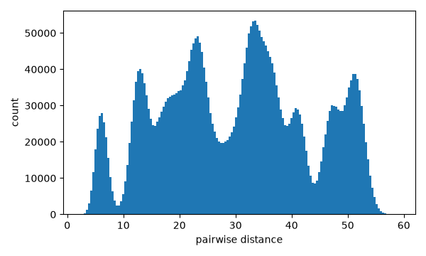
The data imitate a sampled free-energy landscape: 20 Gaussian basins in 16 dimensions, populated unevenly, for around 16000 configurations. The basin centres lie on two concentric rings, so the arrangement the map should recover is known in advance, but every point carries noise in all 16 dimensions.

rng = np.random.default_rng(0)
n_features = 16
n_inner, n_outer = 6, 14

inner_angles = np.linspace(0, 2 * np.pi, n_inner, endpoint=False)
outer_angles = np.linspace(0, 2 * np.pi, n_outer, endpoint=False) + 0.2

centres = np.zeros((n_inner + n_outer, n_features))
centres[:n_inner, 0] = 11 * np.cos(inner_angles)
centres[:n_inner, 1] = 11 * np.sin(inner_angles)
centres[n_inner:, 0] = 26 * np.cos(outer_angles)
centres[n_inner:, 1] = 26 * np.sin(outer_angles)

populations = rng.integers(400, 1200, len(centres))
X = np.vstack(
    [c + rng.normal(0, 1.1, (n, n_features)) for c, n in zip(centres, populations)]
)
basin = np.repeat(np.arange(len(centres)), populations)

fig, ax = plt.subplots(figsize=(6, 3.6))
ax.hist(pdist(X[::6]), bins=150)
ax.set_xlabel("pairwise distance")
ax.set_ylabel("count")
fig.tight_layout()

Landmarks and Voronoi weights#

FPS picks landmarks that are maximally spread out, so on their own they ignore how dense each region is. Weighting every landmark by the number of points in its Voronoi cell (voronoi_weights()) restores that density. Landmarks covering many points get a larger weight. When the full density would drown out sparse but important regions, its power exponent can help to relate the cell populations, interpolating between uniform coverage of the landmarks (power=0) and the density of the full collection (power=1).

fps = FPS(n_to_select=600, random_state=0).fit(X)
landmarks = X[fps.selected_idx_]
landmark_basin = basin[fps.selected_idx_]
weights = voronoi_weights(X, landmarks)

Letting sketch-map choose its parameters#

All five sigmoid parameters default to None, in which case they are estimated from the data, so SketchMap can be fitted without tuning anything. The values it settled on are kept in params_, and passing any of them to the constructor overrides just that one.

sm = SketchMap().fit(landmarks, sample_weight=weights)
for name, value in sm.params_.items():
    print(f"{name:>6} = {value:.3f}")

 sigma = 30.746
a_high = 4.809
b_high = 2.404
 a_low = 2.000
 b_low = 2.000

The estimate reads the parameters off the pairwise distance histogram, placing \(\sigma\) just below its dominant peak. Since the stress sums over pairs with weight \(w_i w_j\), passing sample_weight to fit makes it weight that histogram the same way. FPS spreads its landmarks evenly over the basins, so their unweighted histogram would describe that even spread rather than the populations they stand for. Recomputing the weighted peak by hand shows where \(\sigma\) came from:

distances = cdist(landmarks, landmarks)
upper = np.triu_indices(len(landmarks), k=1)
pair_weights = np.outer(weights, weights)[upper]

bin_edges = np.linspace(0, np.percentile(distances[upper], 99.9), 201)
counts, edges = np.histogram(distances[upper], bins=bin_edges, weights=pair_weights)
centers = 0.5 * (edges[:-1] + edges[1:])
manual_sigma = 0.9 * centers[counts.argmax()]

print(f"weighted-peak sigma by hand: {manual_sigma:.3f}")
print(f"automatic sigma:             {sm.params_['sigma']:.3f}")

weighted-peak sigma by hand: 30.746
automatic sigma:             30.746

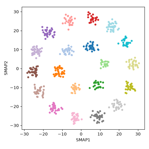
Each point is a landmark, colored by the basin it was drawn from. Every basin comes out as its own island, and the two rings the centres were placed on are recovered from the 16-dimensional cloud.

fig, ax = plt.subplots(figsize=(5, 5))
ax.scatter(
    sm.embedding_[:, 0], sm.embedding_[:, 1], c=landmark_basin, cmap="tab20", s=14
)
ax.set_xlabel("SMAP1")
ax.set_ylabel("SMAP2")
ax.set_aspect("equal", "box")
fig.tight_layout()

Reproducing a published sketch-map#

sketch-map originates from a reference C++ code (sketchmap.org), and the scikit-matter test suite validates this implementation against its output. The strongest check is the protein sketch-map of Ardevol et al., J. Chem. Theory Comput. 2015, 11(3), 1086-1093 (DOI 10.1021/ct500950z). It is 1000 weighted landmarks of 30 Ramachandran angles whose published 2D projection ships with the reference C++. That data is GPL-licensed, so it is not included here and this section is not executed. The recipe and the resulting numbers are reproduced below.

The dihedral angles are periodic, so the distances are computed on the torus and passed in with dissimilarity="precomputed".

By default the embedding is refined with gradient optimization (global_optimizer="gradient"), which is enough for most data. Here we use "grid" instead, which relocates one point at a time as the C++ does. It only works in 2D and is a few times slower, but it escapes minima the gradient cannot, and mixing_schedule="auto" adds the annealing loop of the reference C++ pipeline. That combination is what reaches the published basin below.

raw = np.loadtxt("sketchmap-cpp/examples/protein/lm4.30cv.w01.1")
features, weights = raw[:, :30], raw[:, 30]

delta = np.abs(features[:, None, :] - features[None, :, :])
delta = np.minimum(delta, 2.0 * np.pi - delta)
distances = np.sqrt((delta**2).sum(axis=-1))

sm = SketchMap(
    n_components=2,
    sigma=6.0, a_high=8.0, b_high=8.0, a_low=2.0, b_low=8.0,
    dissimilarity="precomputed",
    global_optimizer="grid",
    mixing_schedule="auto",
)
sm.fit(distances, sample_weight=weights)

The equivalent C++ rerun is utils/sketch-map.sh on lm4.30cv.w01.1, with the inputs from the protein example’s README:

dimensionality of the input data: 30
weighted points: yes, dot-product distances: no, periodicity: 6.283185
high-dimension sigma, a, b: 6 8 8
low-dimension sigma, a, b: 6 2 8

Evaluating our objective at the published coordinates reproduces the C++ stress exactly and fitting from scratch reaches the same basin as the reference pipeline does when it is rerun from scratch:

map	sigmoid stress
published projection, as shipped	0.01596
published projection, locally relaxed	0.00977
C++ `dimred` rerun from scratch	0.00977
skmatter `SketchMap` from scratch	0.00976

The first two rows differ because the published coordinates are not a converged minimum of their own objective: the stress landscape is extremely flat and a plain gradient relaxation started from them (“locally relaxed”) lowers the stress by 39% while barely moving the points. The relaxed value is therefore the depth of the published basin and the number a from-scratch run should be measured against. Even the C++ rerun does not return to the published coordinates exactly, it finds an equally deep minimum with the same structure. The Python fit behaves similarly and its intermediate errors track the C++ annealing ten steps loop round by round.

../../_images/protein_maps.svg — The published projection, the reference C++ rerun and the `SketchMap` fit. Two from-scratch runs agree with each other as closely as either agrees with the published projection.#

References#

Citation [Ceriotti2011] is listed in the References.

Gallery generated by Sphinx-Gallery