Getting started#
This guide illustrates the main functionalities that scikit-matter provides. It
assumes a very basic working knowledge of how scikit-learn works. Please refer to
our Installation instructions for installing scikit-matter.
For a detailed explaination of the functionalities, please look at the Feature and Sample Selection
Features and Samples Selection#
Data sub-selection modules primarily corresponding to methods derived from CUR matrix decomposition and Farthest Point Sampling. In their classical form, CUR and FPS determine a data subset that maximizes the variance (CUR) or distribution (FPS) of the features or samples. These methods can be modified to combine supervised target information denoted by the methods PCov-CUR and PCov-FPS. For further reading, refer to [Imbalzano2018] and [Cersonsky2021]. These selectors can be used for both feature and sample selection, with similar instantiations. All sub-selection methods scores each feature or sample (without an estimator) and chooses that with the maximum score. A simple example of usage:
>>> # feature selection
>>> import numpy as np
>>> from skmatter.feature_selection import CUR, FPS, PCovCUR, PCovFPS
>>> selector = CUR(
...     # the number of selections to make
...     # if None, set to half the samples or features
...     # if float, fraction of the total dataset to select
...     # if int, absolute number of selections to make
...     n_to_select=2,
...     # option to use `tqdm <https://tqdm.github.io/>`_ progress bar
...     progress_bar=True,
...     # float, cutoff score to stop selecting
...     score_threshold=1e-12,
...     # boolean, whether to select randomly after non-redundant selections
...     # are exhausted
...     full=False,
... )
>>> X = np.array(
...     [
...         [0.12, 0.21, 0.02],  # 3 samples, 3 features
...         [-0.09, 0.32, -0.10],
...         [-0.03, -0.53, 0.08],
...     ]
... )
>>> y = np.array([0.0, 0.0, 1.0])  # classes of each sample
>>> selector.fit(X)
CUR(n_to_select=2, progress_bar=True, score_threshold=1e-12)
>>> Xr = selector.transform(X)
>>> print(Xr.shape)
(3, 2)
>>> selector = PCovCUR(n_to_select=2)
>>> selector.fit(X, y)
PCovCUR(n_to_select=2)
>>> Xr = selector.transform(X)
>>> print(Xr.shape)
(3, 2)
>>>
>>> # Now sample selection
>>> from skmatter.sample_selection import CUR, FPS, PCovCUR, PCovFPS
>>> selector = CUR(n_to_select=2)
>>> selector.fit(X)
CUR(n_to_select=2)
>>> Xr = X[selector.selected_idx_]
>>> print(Xr.shape)
(2, 3)
These selectors are available:
CUR: a decomposition: an iterative feature selection method based upon the singular value decoposition.
PCov-CUR decomposition extends upon CUR by using augmented right or left singular vectors inspired by Principal Covariates Regression.
Farthest Point-Sampling (FPS): a common selection technique intended to exploit the diversity of the input space. The selection of the first point is made at random or by a separate metric
PCov-FPS extends upon FPS much like PCov-CUR does to CUR.
Voronoi FPS: conduct FPS selection, taking advantage of Voronoi tessellations to accelerate selection.
Directional Convex Hull (DCH): selects samples by constructing a directional convex hull and determining which samples lie on the bounding surface.
Notebook Examples#

Using scikit-matter selectors with scikit-learn pipelines
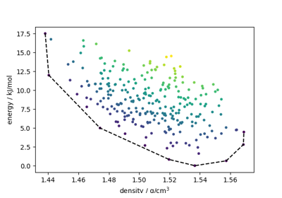
Generalized Convex Hull construction for the polymorphs of ROY

Metrics#
Set of metrics that can be used for an enhanced understanding of your machine learning model.
First are the easily-interpretable error measures of the relative information
capacity of feature space F with respect to feature space F’. The methods
returns a value between 0 and 1, where 0 means that F and F’ are completey
distinct in terms of linearly-decodable information, and where 1 means that F’
is contained in F. All methods are implemented as the root mean-square error
for the regression of the feature matrix X_F’ (or sometimes called Y in the
doc) from X_F (or sometimes called X in the doc) for transformations with
different constraints (linear, orthogonal, locally-linear). By default a custom
2-fold cross-validation skosmo.linear_model.Ridge2FoldCV
is used to ensure the generalization of the transformation and efficiency of the
computation, since we deal with a multi-target regression problem. Methods were
applied to compare different forms of featurizations through different
hyperparameters and induced metrics and kernels [Goscinski2021] .
These reconstruction measures are available:
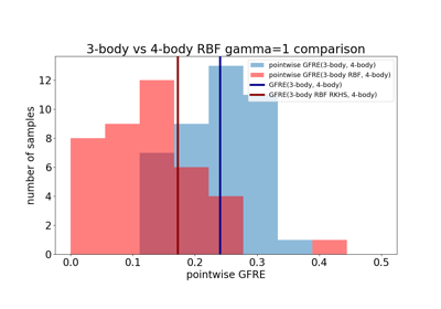
Global Reconstruction Error (GRE) computes the amount of linearly-decodable information recovered through a global linear reconstruction.
Global Reconstruction Distortion (GRD) computes the amount of distortion contained in a global linear reconstruction.
Local Reconstruction Error (LRE) computes the amount of decodable information recovered through a local linear reconstruction for the k-nearest neighborhood of each sample.
Next, we offer a set of prediction rigidity metrics, which can be used to quantify the robustness of the local or component-wise predictions that the machine learning model has been trained to make, based on the training dataset composition.
These prediction rigidities are available:
Local Prediction Rigidity (LPR) computes the local prediction rigidity of a linear or kernel model.
Component-wise Prediction Rigidity (CPR) computes the component-wise prediction rigidity of a linear or kernel model.
There are also two distance metrics compatible with the periodic boundary conditions available.
Note
Currently only rectangular cells are supported. Cell format: [side_length_1, …, side_length_n]
Pairwise Euclidean Distances computes the euclidean distance between two sets of points. It is compatible with the periodic boundary conditions. If the cell length is not provided, it will fall back to the
scikit-learnversion of the euclidean distancesklearn.metrics.pairwise.euclidean_distances().Pairwise Mahalanobis Distance computes the Mahalanobis distance between two sets of points. It is compatible with the periodic boundary conditions.
Notebook Examples#
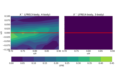

Global Feature Reconstruction Error (GFRE) and Distortion (GFRD)
Hybrid Mapping Techniques#
Often, one wants to construct new ML features from their current representation in order to compress data or visualise trends in the dataset. In the archetypal method for this dimensionality reduction, principal components analysis (PCA), features are transformed into the latent space which best preserves the variance of the original data.
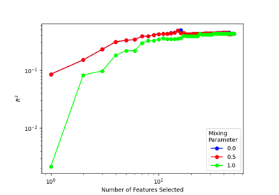
This module provides the Principal Covariates Regression (PCovR), as introduced by [deJong1992], which is a modification to PCA that incorporates target information, such that the resulting embedding could be tuned using a mixing parameter α to improve performance in regression tasks (\(\alpha = 0\) corresponding to linear regression and \(\alpha = 1\) corresponding to PCA). Also provided is Principal Covariates Classification (PCovC), proposed in [Jorgensen2025], which can similarly be used for classification problems.
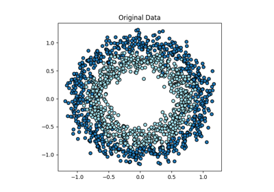
[Helfrecht2020] introduced the non-linear version of PCovR, Kernel Principal Covariates Regression (KPCovR), where the mixing parameter α now interpolates between kernel ridge regression (\(\alpha = 0\)) and kernel principal components analysis (KPCA, \(\alpha = 1\)). A non-linear version of PCovC, Kernel Principal Covariates Classification (KPCovC), is also provided.
The module includes:
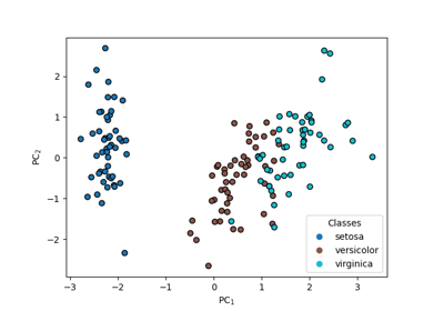
PCovR the standard Principal Covariates Regression. Utilises a combination between a PCA-like and an LR-like loss, and therefore attempts to find a low-dimensional projection of the feature vectors that simultaneously minimises information loss and error in predicting the target properties using only the latent space vectors \(\mathbf{T}\).
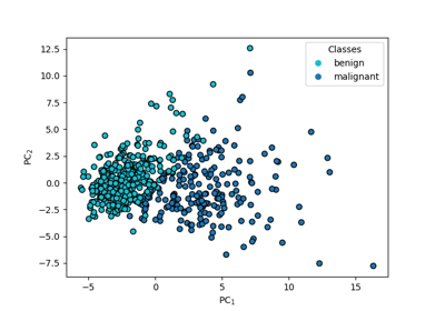
PCovC the standard Principal Covariates Classification, proposed in [Jorgensen2025].
Kernel PCovR the Kernel Principal Covariates Regression. A kernel-based variation on the original PCovR method, proposed in [Helfrecht2020].
Kernel PCovC the Kernel Principal Covariates Classification. A kernel-based modification on the original PCovC method.
Notebook Examples#

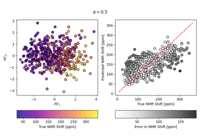

The Importance of Data Scaling in PCovR / KernelPCovR

Gallery generated by Sphinx-Gallery