The Benefits of Kernel PCovR for the WHO Dataset¶

[1]:

import pandas as pd
from matplotlib import pyplot as plt
import numpy as np
from sklearn.linear_model import Ridge, RidgeCV
from sklearn.kernel_ridge import KernelRidge
from sklearn.model_selection import train_test_split
from sklearn.decomposition import PCA, KernelPCA
from sklearn.model_selection import GridSearchCV
from sklearn.metrics import r2_score

from skmatter.preprocessing import StandardFlexibleScaler
from skmatter.decomposition import PCovR, KernelPCovR
from skmatter.datasets import load_who_dataset

from scipy.stats import pearsonr

Load the Dataset¶

[2]:

df = load_who_dataset()['data']
df

[2]:

	Country	Year	SP.POP.TOTL	SH.TBS.INCD	SH.IMM.MEAS	SE.XPD.TOTL.GD.ZS	SH.DYN.AIDS.ZS	SP.DYN.LE00.IN	SH.IMM.IDPT	SH.XPD.CHEX.GD.ZS	SN.ITK.DEFC.ZS	NY.GDP.PCAP.CD
0	Afghanistan	2005	24411191.0	189.0	50.0	2.57000	0.1	58.361	58.0	9.948290	36.1	255.055120
1	Afghanistan	2006	25442944.0	189.0	53.0	2.90000	0.1	58.684	58.0	10.622766	33.3	274.000486
2	Afghanistan	2007	25903301.0	189.0	55.0	2.85000	0.1	59.111	63.0	9.904675	29.8	375.078128
3	Afghanistan	2008	26427199.0	189.0	59.0	3.51000	0.1	59.852	64.0	10.256495	26.5	387.849174
4	Afghanistan	2009	27385307.0	189.0	60.0	3.73000	0.1	60.364	63.0	9.818487	23.3	443.845151
...	...	...	...	...	...	...	...	...	...	...	...	...
2015	South Africa	2015	55876504.0	988.0	86.0	5.48285	18.2	63.950	85.0	8.790190	5.2	6204.929901
2016	South Africa	2016	56422274.0	805.0	84.0	5.44424	18.4	64.747	85.0	8.821429	5.4	5735.066787
2017	South Africa	2017	56641209.0	738.0	81.0	5.59867	18.5	65.402	84.0	8.722624	5.5	6734.475153
2018	South Africa	2018	57339635.0	677.0	81.0	5.64401	18.6	65.674	82.0	8.858297	5.7	7048.522211
2019	South Africa	2019	58087055.0	615.0	83.0	5.91771	18.6	66.175	85.0	9.109355	6.3	6688.787271

2020 rows × 12 columns

[3]:

columns = [
    "SP.POP.TOTL",
    "SH.TBS.INCD",
    "SH.IMM.MEAS",
    "SE.XPD.TOTL.GD.ZS",
    "SH.DYN.AIDS.ZS",
    "SH.IMM.IDPT",
    "SH.XPD.CHEX.GD.ZS",
    "SN.ITK.DEFC.ZS",
    "NY.GDP.PCAP.CD",
]

X_raw = np.array(df[columns])

# We are taking the logarithm of the population  and GDP to avoid extreme distributions
log_scaled = ["SP.POP.TOTL", "NY.GDP.PCAP.CD"]
for ls in log_scaled:
    print(X_raw[:, columns.index(ls)].min(), X_raw[:, columns.index(ls)].max())
    if ls in columns:
        X_raw[:, columns.index(ls)] = np.log10(X_raw[:, columns.index(ls)])
y_raw = np.array(df["SP.DYN.LE00.IN"])  # [np.where(df['Year']==2000)[0]])
y_raw = y_raw.reshape(-1, 1)
X_raw.shape

149841.0 7742681934.0
110.460874721483 123678.70214327476

[3]:

(2020, 9)

Scale and Center the Features and Targets¶

[4]:

x_scaler = StandardFlexibleScaler(column_wise=True)
X = x_scaler.fit_transform(X_raw)

y_scaler = StandardFlexibleScaler(column_wise=True)
y = y_scaler.fit_transform(y_raw)

n_components = 2

X_train, X_test, y_train, y_test = train_test_split(X, y, test_size=0.3, shuffle=True, random_state=0)

Train the Different Linear DR Techniques¶

[5]:

# Best Error for Linear Regression
RidgeCV(cv=5, alphas=np.logspace(-8,2, 20), fit_intercept=False).fit(X_train, y_train).score(X_test, y_test)

[5]:

0.8548848257886273

PCovR¶

[6]:

pcovr = PCovR(n_components=n_components, regressor=Ridge(alpha=1e-4, fit_intercept=False), mixing=0.5, random_state=0).fit(X_train, y_train)
T_train_pcovr = pcovr.transform(X_train)
T_test_pcovr = pcovr.transform(X_test)
T_pcovr = pcovr.transform(X)

r_pcovr = Ridge(alpha=1e-4, fit_intercept=False, random_state=0).fit(T_train_pcovr, y_train)
yp_pcovr = r_pcovr.predict(T_test_pcovr)

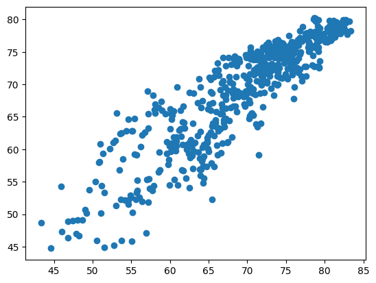
plt.scatter(y_scaler.inverse_transform(y_test), y_scaler.inverse_transform(yp_pcovr))
r_pcovr.score(T_test_pcovr, y_test)

/home/docs/checkouts/readthedocs.org/user_builds/scikit-matter/envs/v0.1.4/lib/python3.8/site-packages/skmatter/decomposition/_pcovr.py:274: UserWarning: This class does not automatically center data, and your data mean is greater than the supplied tolerance.
  warnings.warn(

[6]:

0.8267220275787428

../_images/read-only-examples_PCovR-WHODataset_10_2.png

PCA¶

[7]:

pca = PCA(
    n_components=n_components, random_state=0,
).fit(X_train, y_train)
T_train_pca = pca.transform(X_train)
T_test_pca = pca.transform(X_test)
T_pca = pca.transform(X)

r_pca = Ridge(alpha=1e-4, fit_intercept=False, random_state=0).fit(T_train_pca, y_train)
yp_pca = r_pca.predict(T_test_pca)

plt.scatter(y_scaler.inverse_transform(y_test), y_scaler.inverse_transform(yp_pca))
r_pca.score(T_test_pca, y_test)

[7]:

0.8041174131375703

../_images/read-only-examples_PCovR-WHODataset_12_1.png

[8]:

for c, x in zip(columns, X.T):
    print(c, pearsonr(x, T_pca[:,0])[0], pearsonr(x, T_pca[:,1])[0])

SP.POP.TOTL 0.22694404485361105 -0.3777743593940674
SH.TBS.INCD 0.6249287177098696 0.631621515170247
SH.IMM.MEAS -0.8425862283813432 0.1360690482747245
SE.XPD.TOTL.GD.ZS -0.41457342404840203 0.6100854823971242
SH.DYN.AIDS.ZS 0.3260933054303088 0.8499296260662156
SH.IMM.IDPT -0.8422637385674647 0.16339769662914994
SH.XPD.CHEX.GD.ZS -0.4590012089554527 0.3068630393788181
SN.ITK.DEFC.ZS 0.8212324937958551 0.05510883584395285
NY.GDP.PCAP.CD -0.8042167907410391 0.06566227478694735

Train the Different Kernel DR Techniques¶

Select Kernel Hyperparameters¶

[9]:

param_grid = {"gamma": np.logspace(-8, 3, 20), "alpha": np.logspace(-8, 3, 20)}
clf = KernelRidge(kernel='rbf')

gs = GridSearchCV(estimator=clf, param_grid=param_grid)
gs.fit(X_train, y_train)
gs.best_estimator_

[9]:

KernelRidge(alpha=0.0016237767391887243, gamma=0.08858667904100832,
            kernel='rbf')

In a Jupyter environment, please rerun this cell to show the HTML representation or trust the notebook.
On GitHub, the HTML representation is unable to render, please try loading this page with nbviewer.org.

[10]:

# Best Error for Kernel Regression
gs.best_score_

[10]:

0.971744613370008

[11]:

kernel_params = {"kernel": "rbf", "gamma": gs.best_estimator_.gamma}

KPCovR¶

[12]:

kpcovr = KernelPCovR(
    n_components=n_components,
    regressor=KernelRidge(alpha=gs.best_estimator_.alpha, **kernel_params),
    mixing=0.5,
    **kernel_params,
).fit(X_train, y_train)

T_train_kpcovr = kpcovr.transform(X_train)
T_test_kpcovr = kpcovr.transform(X_test)
T_kpcovr = kpcovr.transform(X)

r_kpcovr = KernelRidge(**kernel_params).fit(T_train_kpcovr, y_train)
yp_kpcovr = r_kpcovr.predict(T_test_kpcovr)

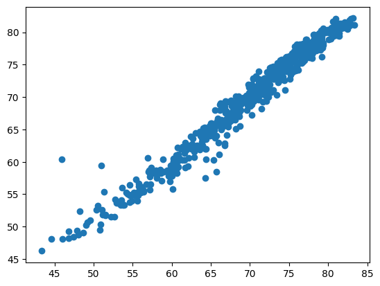
plt.scatter(y_scaler.inverse_transform(y_test), y_scaler.inverse_transform(yp_kpcovr))
r_kpcovr.score(T_test_kpcovr, y_test)

[12]:

0.9701003539459829

../_images/read-only-examples_PCovR-WHODataset_20_1.png

KPCA¶

[13]:

kpca = KernelPCA(
    n_components=n_components,
    **kernel_params,
    random_state=0
).fit(X_train, y_train)

T_train_kpca = kpca.transform(X_train)
T_test_kpca = kpca.transform(X_test)
T_kpca = kpca.transform(X)

r_kpca = KernelRidge(**kernel_params).fit(T_train_kpca, y_train)
yp_kpca = r_kpca.predict(T_test_kpca)

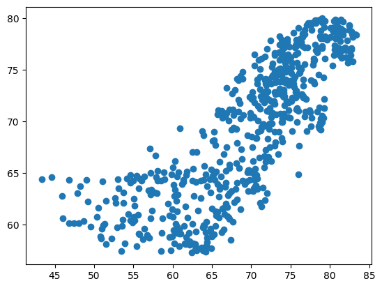
plt.scatter(y_scaler.inverse_transform(y_test), y_scaler.inverse_transform(yp_kpca))
r_kpca.score(T_test_kpca, y_test)

[13]:

0.6661226058827701

../_images/read-only-examples_PCovR-WHODataset_22_1.png

Correlation of the different variables with the KPCovR axes¶

[14]:

for c, x in zip(columns, X.T):
    print(c, pearsonr(x, T_kpcovr[:,0])[0], pearsonr(x, T_kpcovr[:,1])[0])

SP.POP.TOTL 0.07320109486752663 0.03969226130206769
SH.TBS.INCD 0.6836177728806969 -0.053847467712589955
SH.IMM.MEAS -0.6604939713031328 0.047519698516421745
SE.XPD.TOTL.GD.ZS -0.2300978893002612 -0.36227488660047863
SH.DYN.AIDS.ZS 0.5157981075022106 -0.11701327000167581
SH.IMM.IDPT -0.6449500965013223 0.052622267816944665
SH.XPD.CHEX.GD.ZS -0.38019935560128637 -0.5736426627630692
SN.ITK.DEFC.ZS 0.7301250686596606 0.04793454286931878
NY.GDP.PCAP.CD -0.822866009733033 -0.4938636569729072

Plot Our Results¶

[15]:

fig, axes = plt.subplot_mosaic(
    """
                                AFF.B
                                A.GGB
                                .....
                                CHH.D
                                C.IID
                                .....
                                EEEEE
                                """,
    figsize=(7.5, 7.5),
    gridspec_kw=dict(
        height_ratios=(0.5, 0.5, 0.1, 0.5, 0.5, 0.1, 0.1),
        width_ratios=(1, 0.1, 0.2, 0.1, 1)
    ),
)
axPCA, axPCovR, axKPCA, axKPCovR = axes["A"], axes["B"], axes["C"], axes["D"]
axPCAy, axPCovRy, axKPCAy, axKPCovRy = axes["F"], axes["G"], axes["H"], axes["I"]

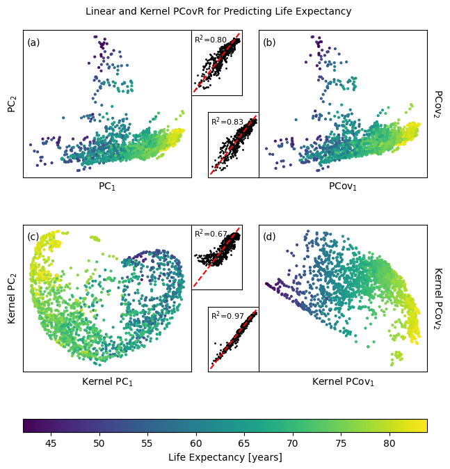
def add_subplot(ax, axy, T, yp, let=''):
    p = ax.scatter(-T[:, 0], T[:, 1], c=y_raw, s=4)
    ax.set_xticks([])
    ax.set_yticks([])
    ax.annotate(
        xy=(0.025, 0.95),
        xycoords="axes fraction",
        text=f"({let})",
        va='top',
        ha='left'
    )
    axy.scatter(
        y_scaler.inverse_transform(y_test),
        y_scaler.inverse_transform(yp),
        c="k",
        s=1,
    )
    axy.plot([y_raw.min(), y_raw.max()], [y_raw.min(), y_raw.max()], "r--")
    axy.annotate(
        xy=(0.05, 0.95),
        xycoords="axes fraction",
        text=r"R$^2$=%0.2f" % round(r2_score(y_test, yp), 3),
        va='top',
        ha='left',
        fontsize=8,
    )
    axy.set_xticks([])
    axy.set_yticks([])
    return p


p = add_subplot(axPCA, axPCAy, T_pca, yp_pca, 'a')
axPCA.set_xlabel("PC$_1$")
axPCA.set_ylabel("PC$_2$")

add_subplot(axPCovR, axPCovRy, T_pcovr @ np.diag([-1,1]), yp_pcovr, 'b')
axPCovR.yaxis.set_label_position("right")
axPCovR.set_xlabel("PCov$_1$")
axPCovR.set_ylabel("PCov$_2$", rotation=-90, va="bottom")

add_subplot(axKPCA, axKPCAy, T_kpca @ np.diag([-1,1]), yp_kpca, 'c')
axKPCA.set_xlabel("Kernel PC$_1$", fontsize=10)
axKPCA.set_ylabel("Kernel PC$_2$", fontsize=10)

add_subplot(axKPCovR, axKPCovRy, T_kpcovr, yp_kpcovr, 'd')
axKPCovR.yaxis.set_label_position("right")
axKPCovR.set_xlabel("Kernel PCov$_1$", fontsize=10)
axKPCovR.set_ylabel("Kernel PCov$_2$", rotation=-90, va="bottom", fontsize=10)

plt.colorbar(
    p, cax=axes["E"], label="Life Expectancy [years]", orientation="horizontal"
)
fig.subplots_adjust(wspace=0, hspace=0.4)
fig.suptitle("Linear and Kernel PCovR for Predicting Life Expectancy", y=0.925, fontsize=10)
plt.show()

../_images/read-only-examples_PCovR-WHODataset_26_0.png