Choosing Different Regressors for PCovR

from sklearn.datasets import load_diabetes

from matplotlib import pyplot as plt

from skmatter.decomposition import PCovR
from sklearn.preprocessing import StandardScaler
from sklearn.linear_model import Ridge

For this, we will use the diabetes dataset from sklearn.

mixing = 0.5

X, y = load_diabetes(return_X_y=True)
y = y.reshape(X.shape[0], -1)

X_scaler = StandardScaler()
X_scaled = X_scaler.fit_transform(X)

y_scaler = StandardScaler()
y_scaled = y_scaler.fit_transform(y)

Use the default regressor in PCovR

When there is no regressor supplied, PCovR uses sklearn.linear_model.Ridge('alpha':1e-6, 'fit_intercept':False, 'tol':1e-12).

%%time
pcovr1 = PCovR(
    mixing=mixing,
    n_components=2,
)
pcovr1.fit(X_scaled, y_scaled)
print("Regressor is", pcovr1.regressor_, "\n")

Regressor is Ridge(alpha=1e-06, fit_intercept=False, tol=1e-12)

CPU times: user 9.62 ms, sys: 155 µs, total: 9.78 ms
Wall time: 9.78 ms

Use a fitted regressor

You can pass a fitted regressor to PCovR to rely on the predetermined regression parameters. Currently, scikit-matter supports scikit-learn classes LinearModel, Ridge, and RidgeCV, with plans to support anu regressor with similar architecture in the future.

%%time
regressor = Ridge(alpha=1e-6, fit_intercept=False, tol=1e-12).fit(X_scaled, y_scaled)

CPU times: user 1.07 ms, sys: 0 ns, total: 1.07 ms
Wall time: 1.07 ms

%%time
pcovr2 = PCovR(
    mixing=mixing,
    n_components=2,
    regressor=regressor
)
pcovr2.fit(X_scaled, y_scaled)
print("Regressor is", pcovr2.regressor_, "\n")

Regressor is Ridge(alpha=1e-06, fit_intercept=False, tol=1e-12)

CPU times: user 7.3 ms, sys: 0 ns, total: 7.3 ms
Wall time: 7.31 ms

Use a pre-predicted y

With regressor='precomputed', you can pass a regression output \(\hat{Y}\) and optional regression weights \(W\) to PCovR. If W=None, then PCovR will determine \(W\) as the least-squares solution between \(X\) and \(\hat{Y}\).

%%time
regressor = Ridge(alpha=1e-6, fit_intercept=False, tol=1e-12).fit(X_scaled, y_scaled)
Yhat = regressor.predict(X_scaled)
W = regressor.coef_

CPU times: user 1.14 ms, sys: 107 µs, total: 1.25 ms
Wall time: 1.25 ms

%%time
pcovr3 = PCovR(
    mixing=mixing,
    n_components=2,
    regressor='precomputed'
)
pcovr3.fit(X_scaled, y_scaled, W=W)

CPU times: user 3.98 ms, sys: 0 ns, total: 3.98 ms
Wall time: 3.98 ms

PCovR(n_components=2, regressor='precomputed', space='feature')

In a Jupyter environment, please rerun this cell to show the HTML representation or trust the notebook.
On GitHub, the HTML representation is unable to render, please try loading this page with nbviewer.org.

Comparing Results

Because we used the same regressor in all three models, they will yield the same result.

fig, (ax1, ax2, ax3) = plt.subplots(1,
                                    3,
                                    figsize=(12, 4),
                                    sharex=True,
                                    sharey=True)

ax1.scatter(*pcovr1.transform(X_scaled).T, c=y)
ax2.scatter(*pcovr2.transform(X_scaled).T, c=y)
ax3.scatter(*pcovr3.transform(X_scaled).T, c=y)

ax1.set_ylabel("PCov$_2$")
ax1.set_xlabel("PCov$_1$")
ax2.set_xlabel("PCov$_1$")
ax3.set_xlabel("PCov$_1$")

ax1.set_title("Default Regressor")
ax2.set_title("Pre-fit Regressor")
ax3.set_title("Precomputed Regression Result")

Text(0.5, 1.0, 'Precomputed Regression Result')

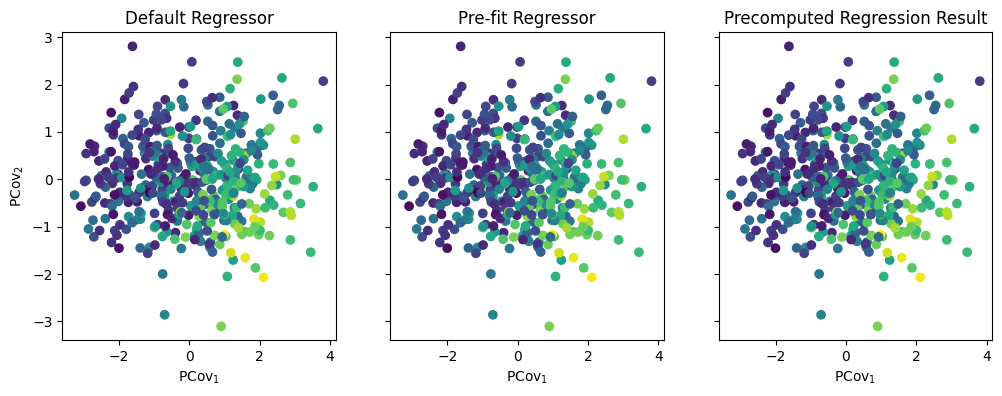
As you can imagine, these three options have different use cases – if you are working with a large dataset, you should always pre-fit to save on time!