The Importance of Data Scaling in PCovR / KernelPCovR

import numpy as np
from matplotlib import pyplot as plt

from sklearn.datasets import load_diabetes
from sklearn.preprocessing import StandardScaler
from skmatter.preprocessing import StandardFlexibleScaler
from skmatter.decomposition import PCovR

In PCovR, and KernelPCovR, we are combining multiple aspects of the dataset, primarily the features and targets. As such, the results largely depend on the relative contributions of each aspect to the mixed model.

X, y = load_diabetes(return_X_y=True)

Take the diabetes dataset from sklearn. In their raw form, the magnitudes of the features and targets are

print(
    "Norm of the features: %0.2f \nNorm of the targets: %0.2f"
    % (np.linalg.norm(X), np.linalg.norm(y))
)

Norm of the features: 3.16
Norm of the targets: 3584.82

For the California dataset, we can use the StandardScaler class from sklearn, as the features and targets are independent.

x_scaler = StandardScaler()
y_scaler = StandardScaler()

X_scaled = x_scaler.fit_transform(X)
y_scaled = y_scaler.fit_transform(y.reshape(-1,1))

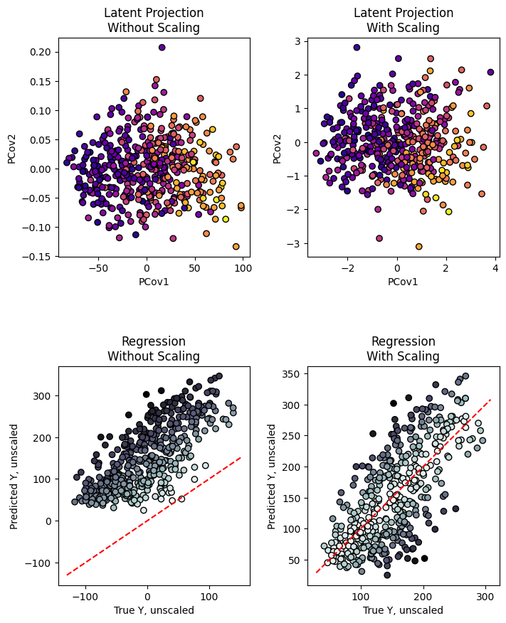
Looking at the results at mixing=0.5, we see an especially large difference in the latent-space projections

pcovr_unscaled = PCovR(mixing=0.5, n_components=4).fit(X, y)
T_unscaled = pcovr_unscaled.transform(X)
Yp_unscaled = pcovr_unscaled.predict(X)

pcovr_scaled = PCovR(mixing=0.5, n_components=4).fit(X_scaled, y_scaled)
T_scaled = pcovr_scaled.transform(X_scaled)
Yp_scaled = y_scaler.inverse_transform(pcovr_scaled.predict(X_scaled))

fig, ((ax1_T, ax2_T), (ax1_Y, ax2_Y)) = plt.subplots(2, 2, figsize=(8, 10))

ax1_T.scatter(T_unscaled[:, 0], T_unscaled[:, 1], c=y, cmap="plasma", ec="k")
ax1_T.set_xlabel("PCov1")
ax1_T.set_ylabel("PCov2")
ax1_T.set_title("Latent Projection\nWithout Scaling")

ax2_T.scatter(T_scaled[:, 0], T_scaled[:, 1], c=y, cmap="plasma", ec="k")
ax2_T.set_xlabel("PCov1")
ax2_T.set_ylabel("PCov2")
ax2_T.set_title("Latent Projection\nWith Scaling")

ax1_Y.scatter(Yp_unscaled, y, c=np.abs(y - Yp_unscaled), cmap="bone_r", ec="k")
ax1_Y.plot(ax1_Y.get_xlim(), ax1_Y.get_xlim(), "r--")
ax1_Y.set_xlabel("True Y, unscaled")
ax1_Y.set_ylabel("Predicted Y, unscaled")
ax1_Y.set_title("Regression\nWithout Scaling")

ax2_Y.scatter(Yp_scaled,
              y,
              c=np.abs(y.flatten() - Yp_scaled.flatten()),
              cmap="bone_r",
              ec="k")
ax2_Y.plot(ax2_Y.get_xlim(), ax2_Y.get_xlim(), "r--")
ax2_Y.set_xlabel("True Y, unscaled")
ax2_Y.set_ylabel("Predicted Y, unscaled")
ax2_Y.set_title("Regression\nWith Scaling")

fig.subplots_adjust(hspace=0.5, wspace=0.3)

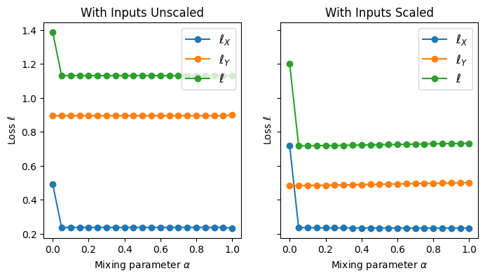
Also, we see that when the datasets are unscaled, the total loss (loss in recreating the original dataset and regression loss) does not vary with mixing, as expected. Typically, the regression loss should gradually increase with mixing (and vice-versa for the loss in reconstructing the original features). When the inputs are not scaled, however, only in the case of mixing = 0 or 1 will the losses drastically change, depending on which component is dominating the model. Here, because the features dominate the model, this jump occurs as mixing goes to 0. With the scaled inputs, there is still a jump when mixing>0 due to the change in matrix rank.

mixings = np.linspace(0, 1, 21)
losses_unscaled = np.zeros((2, len(mixings)))
losses_scaled = np.zeros((2, len(mixings)))

nc = 4

for mi, mixing in enumerate(mixings):
    pcovr_unscaled = PCovR(mixing=mixing, n_components=nc).fit(X, y)
    t_unscaled = pcovr_unscaled.transform(X)
    yp_unscaled = pcovr_unscaled.predict(T=t_unscaled)
    xr_unscaled = pcovr_unscaled.inverse_transform(t_unscaled)
    losses_unscaled[:, mi] = (
        np.linalg.norm(xr_unscaled - X)**2.0 / np.linalg.norm(X)**2,
        np.linalg.norm(yp_unscaled - y)**2.0 / np.linalg.norm(y)**2,
    )

    pcovr_scaled = PCovR(mixing=mixing, n_components=nc).fit(X_scaled, y_scaled)
    t_scaled = pcovr_scaled.transform(X_scaled)
    yp_scaled = pcovr_scaled.predict(T=t_scaled)
    xr_scaled = pcovr_scaled.inverse_transform(t_scaled)
    losses_scaled[:, mi] = (
        np.linalg.norm(xr_scaled - X_scaled)**2.0 /
        np.linalg.norm(X_scaled)**2,
        np.linalg.norm(yp_scaled - y_scaled)**2.0 /
        np.linalg.norm(y_scaled)**2,
    )

fig, (ax1, ax2) = plt.subplots(1, 2, figsize=(8, 4), sharey=True, sharex=True)
ax1.plot(mixings, losses_unscaled[0], marker="o", label=r"$\ell_{X}$")
ax1.plot(mixings, losses_unscaled[1], marker="o", label=r"$\ell_{Y}$")
ax1.plot(mixings,
             np.sum(losses_unscaled, axis=0),
             marker="o",
             label=r"$\ell$")
ax1.legend(fontsize=12)
ax1.set_title('With Inputs Unscaled')
ax1.set_xlabel(r'Mixing parameter $\alpha$')
ax1.set_ylabel(r'Loss $\ell$')

ax2.plot(mixings, losses_scaled[0], marker="o", label=r"$\ell_{X}$")
ax2.plot(mixings, losses_scaled[1], marker="o", label=r"$\ell_{Y}$")
ax2.plot(mixings,
             np.sum(losses_scaled, axis=0),
             marker="o",
             label=r"$\ell$")
ax2.legend(fontsize=12)
ax2.set_title('With Inputs Scaled')
ax2.set_xlabel(r'Mixing parameter $\alpha$')
ax2.set_ylabel(r'Loss $\ell$')

Text(0, 0.5, 'Loss $\\ell$')

Note: when the relative magnitude of the features or targets is important, such as in load_csd_1000r, one should use the ``StandardFlexibleScaler`` provided by ``scikit-matter``.